Architecture of mavkit-snoop
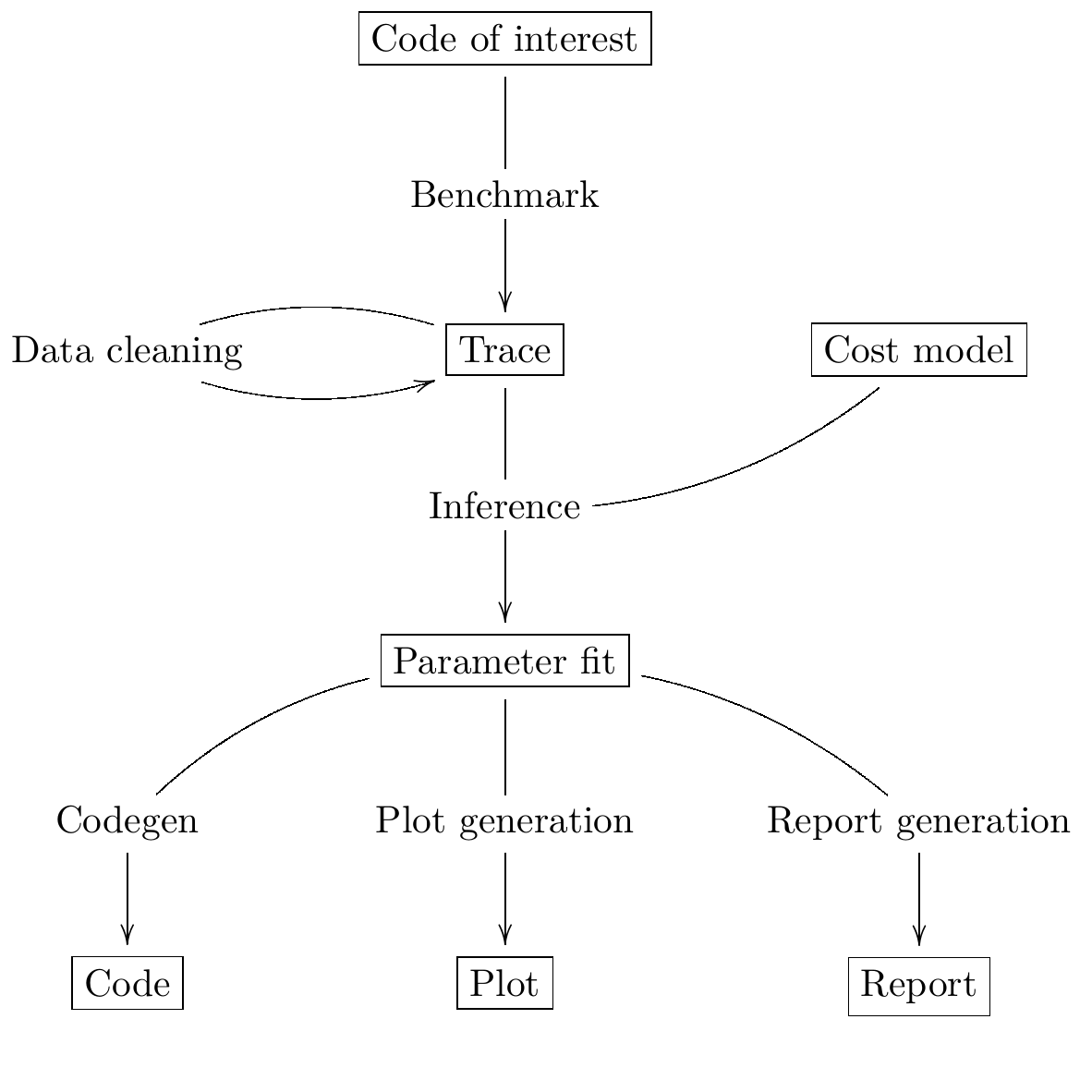
The following figure describes the main functionalities and data
processed by mavkit-snoop, to be read from top to bottom. The boxed
nodes represents the various kinds of data processed by the tool,
while the unboxed items represent computational steps.
The code architecture of mavkit-snoop is itself divided in the following
main packages:
bin_snoopis the main binary (you can have a look at the manual).mavryk-benchmarkis a library for performing measurements, writing models and infering parameters for these models.mavryk-micheline-rewritingis used to perform rewriting of Micheline terms (documentation available here). It is mainly used when writing protocol-specific benchmarks but is independent from the protocol.
There are other packages containing shell-specific and protocol-specific benchmarks, these are not documented here.
Here, we will focus on the mavryk-benchmark library, which is the core of the
tool.
High-level description
mavkit-snoop is a tool for benchmarking and fitting statistical models which predict the performance of any piece of code of interest.
More concretely, let us consider a piece of code for which we wish to predict its performance. To understand the performance profile of this piece of code, we must execute it with different arguments, varying the size of the problem to be solved. As “the size of the problem to be solved” is a long expression, we will use the shorter term workload for that.
The notion of workload is abstract here, and indeed, it is not necessarily a scalar. Here are a few examples of workloads:
Timer benchmarks measure the latency of the timer itself and the associated workloads record nothing.
IO benchmarks measure the execution time of performing specific read and write patterns to the underlying key-value store and the associated workloads record the size of the storage as well as the parameters (bytes read/written, length of keys, etc) of these accesses.
Translator benchmarks measure the execution time of various pieces of
Script_ir_translator(the translator for short, which handles typechecking/unparsing of code and data) as well as Micheline serialization, and corresponding workloads record the size of the typechecked/unparsed/(de)serialized terms.Michelson benchmarks measure the execution time of the interpreter on specific programs and the associated workloads record the list of all executed instructions together with, for each instruction, the sizes of the operands as encountered on the stack.
Once this notion of workload is clear, we can describe Snoop’s user interface.
Using mavryk-benchmark requires to provide, for each benchmark, the following main items:
a type of execution
workload;a statistical model, corresponding to a function which to each
workloadassociates an expression (possibly with free variables) denoting the predicted execution time for that workload. In simple cases, the model consists in a single expression computing a predicted execution time for any given workload.A family of pieces of code (i.e. closures) to be benchmarked, each associated to its
workload. Thus, each closure contains the application of a piece of a code to arguments instantiating a specific workload. We assume that the execution time of each closure has a well-defined distribution. In most cases, these closures correspond to executing a single piece of code of interest with different inputs.
From this input, mavryk-benchmark can perform for you the following tasks:
perform the timing measurements;
infer the free parameters of the statistical model;
display the results of benchmarking and inference;
generate code from the model.
Code organization
The data type that wraps everything up is the module type Benchmark.S.
The main items required by this type are:
create_benchmarks, a function that must generate closures and their associated workloads (packed together in type'workload Generator.benchmark).models, a list of statistical models that we’d like to fit to predict the execution time of the piece of code of interest.
The library is meant to be used as follows:
define a
Benchmark.S, which requiresconstructing benchmarks
defining models, either pre-built (via the
Modelmodule) or from scratch (using theCostlangDSL);
generate empirical timing measurements using
Measure.perform_benchmark;given the data generated, infer parameters of the models using
Inference.make_problemandInference.solve_problem;exploit the results:
input back the result of inference in the model to make it predictive
plot the data (
mavryk-benchmarkcan generate CSV)generate code from the model (
Codegenmodule)
Modules implementing the Benchmark.S signature can also be registered
via the Registration.register function which makes them available to
mavkit-snoop, a binary that wraps these features under a nice CLI.
Defining benchmarks: the Generator module
The Generator.benchmark type defines the interface that each benchmark
must implement. At the time of writing, this type specifies three ways
to provide a benchmark (but more could easily be added):
type 'workload benchmark =
  | Plain : {workload : 'workload; closure : unit -> unit} -> 'workload benchmark
  | With_context : {
      workload : 'workload;
      closure : 'context -> unit;
      with_context : 'a. ('context -> 'a) -> 'a;
    } -> 'workload benchmark
  | With_probe : {
      workload : 'aspect -> 'workload;
      probe : 'aspect probe;
      closure : 'aspect probe -> unit;
    }
      -> 'workload benchmark
Plain benchmarks
The Plain constructor simply packs a workload and a closure together.
The implied semantics of this benchmark is that the closure is
a stateless piece of code, ready to be executed thousands of times
by the measure infrastructure.
With_context benchmarks
The With_context constructor allows to define benchmarks we
require to set up and cleanup a context, shared by all executions of
the closure. An example (which prompted the addition of this feature)
is the case of storage benchmarks, where we need to create a directory
and set up some files before executing a closure containing e.g.
a read or write access, after which the directory must be removed.
With_probe benchmarks
The With_probe constructor allows fine-grained benchmarking by
inverting control: the user is in charge of calling the pieces of code
to be benchmarked using the provided probe. The definition of a
probe consists in a small object with three methods:
type 'aspect probe = {
  apply : 'a. 'aspect -> (unit -> 'a) -> 'a;
  aspects : unit -> 'aspect list;
  get : 'aspect -> float list;
}
The intended semantics of each method is as follows:
calling
probe.apply aspect fexecutesf, performing e.g. a timing measurement off’s execution time and returns the result of the evaluation. The measurement is associated to the specifiedaspectin a side-effecting way.probe.aspectsreturns the list of all aspects.Finally,
probe.get aspectreturns all the measurements associated toaspect.
Note that With_probe benchmarks do not come with a fixed workload,
but rather with an aspect-indexed family of workloads. This reflects
the fact that this kind of benchmark can measure
several different pieces of code in the same run,
each potentially associated to its own cost model.
The function Measure.make_timing_probe provides a basic probe
implementation. The unit test in src/lib_benchmark/test/test_probe.ml
contains an example.
Defining a predictive model: the Model module
As written above, the Benchmark.S signature also requires a list
of models (note that users only interested in measures of execution
time can leave this list empty). At the time of writing, mavryk-benchmark
only handles linear models.
Linear models: a primer
We aim at predicting the cost (typically, execution time) for various parts of the codebase. To do this, we must first come up with a model. These cost models take as input some notion of “size” (typically a vector of integers) and output a prediction of execution time (or, up to unit conversion, a quantity of gas). If \(S\) is the abstract set of sizes, we’re trying to infer a function of type \(S \rightarrow \mathbb{R}_{\ge 0}\) from a finite list of examples \((s_n, t_n)_n \in (S \times \mathbb{R}_{\ge 0})^\ast\) which minimizes some error criterion. This is an example of a regression problem.
Note that since \(S\) is typically not finite, \(S \rightarrow \mathbb{R}_{\ge 0}\) is an infinite-dimensional vector space. We will restrict our search to a \(n\)-dimensional subset of functions \(f_\theta\), with \(\theta \in \mathbb{R}^n\), of the form
where the \((g_i)_{i=1}^n\) is a fixed family of functions \(g_i : S \rightarrow \mathbb{R}_{\ge 0}\). An \(n\)-dimensional linear cost model is entirely determined by the \(g_i\).
Enumerating the currying isomorphisms, a linear model can be considered as:
a linear function \(\mathbb{R}^n \multimap (S \rightarrow \mathbb{R}_{\ge 0})\) from “meta” parameters to cost functions;
a function \(S \rightarrow (\mathbb{R}^n \rightarrow \mathbb{R}_{\ge 0})\) from sizes to linear forms over “meta” parameters;
a function \(S \times \mathbb{R}^n \rightarrow \mathbb{R}_{\ge 0}\).
The two first forms are the useful ones. The first form is useful in stating the inference problem: we seek \(\theta\) that minimizes some empirical error measure over the benchmark results. The second form is useful as it allows to transform the linear model in vector form, when applying the size.
The Costlang DSL
The module Costlang defines a small language in which to define terms
having both free and bound variables. The intended semantics for free
variables is to stand in for variables to be inferred during the inference
process (corresponding to \(\theta_i\) in the previous section).
The language is defined in tagless final style. If this does not
ring a bell, we strongly recommend you take a look at
https://okmij.org/ftp/tagless-final/index.html in order to make sense of the
rest of this section. The syntax is specified by the Costlang.S module
type:
module type S = sig
  type 'a repr
  type size
  val true_ : bool repr
  val false_ : bool repr
  val int : int -> size repr
  val float : float -> size repr
  val ( + ) : size repr -> size repr -> size repr
  val ( - ) : size repr -> size repr -> size repr
  val ( * ) : size repr -> size repr -> size repr
  val ( / ) : size repr -> size repr -> size repr
  val max : size repr -> size repr -> size repr
  val min : size repr -> size repr -> size repr
  val log2 : size repr -> size repr
  val free : name:Free_variable.t -> size repr
  val lt : size repr -> size repr -> bool repr
  val eq : size repr -> size repr -> bool repr
  val shift_left : size repr -> int -> size repr
  val shift_right : size repr -> int -> size repr
  val lam : name:string -> ('a repr -> 'b repr) -> ('a -> 'b) repr
  val app : ('a -> 'b) repr -> 'a repr -> 'b repr
  val let_ : name:string -> 'a repr -> ('a repr -> 'b repr) -> 'b repr
  val if_ : bool repr -> 'a repr -> 'a repr -> 'a repr
end
In a nutshell, the type of terms is type 'a term = \pi (X : S). 'a X.repr,
i.e. terms must be thought of as parametric in their implementation,
provided by a module of type S.
It must be noted that this language does not enforce that built
terms are linear (in the usual, not type-theoretic sense) in their
free variables: this invariant must be currently enforced dynamically.
The Costlang module defines some useful functions for manipulating
terms and printing terms:
Costlang.Pp_implis a simple pretty printer,Costang.Eval_implis an evaluator (which fails on terms having free variables),Costlang.Eval_linear_combination_implevaluates terms which are linear combinations in their free variables to vectors (corresponding to applying a size parameter to the second curried form in the previous section),Costlang.Substallows to perform substitution of free variables,Costlang.Hash_consallows to manipulate hash-consed terms,Costlang.Beta_normalizeallows to beta-normalize…
Other implementations are provided elsewhere, e.g. for code or report generation.
Definition of cost models: the Model module
The Model module provides a higher-level interface over Costlang,
and pre-defines widely used models. These pre-defined models are independent
of any specific workload: they need to be packaged together with a conversion
function from the workload of the benchmark of interest to the domain
of the model. The Model.make ~conv ~model function does just this.
The Measure module
The Measure module is dedicated to measuring the execution
time of closures held in Generator.benchmark values and
turn these into timed workloads (i.e. pairs of workload and execution time).
It also contains routines to remove outliers and to save and load
workload data together with extra metadata.
Measuring execution time of Generator.benchmark values
The core of the functionality is provided by the Measure.perform_benchmark
function.
val perform_benchmark :
  Measure.options -> ('c, 't) Mavryk_benchmark.Benchmark.poly -> 't workload_data
Before delving into its implementation, let’s examine its type.
A value of type ('c, 't) Mavryk_benchmark.Benchmark.poly is a first
class module where 'c is a type variable corresponding to the configuration
of the benchmark and 't is a variable corresponding to the type
of workloads of the benchmark. Hence perform_benchmark is parametric
in these types.
Under the hood, this functions calls to the create_benchmarks
function provided by the first class module to create a list of
Generator.benchmark values. This might involve loading from
benchmark-specific parameters from a JSON file if the benchmark
so requires. After setting up some benchmark parameters
(random seed, GC parameters, CPU affinity), the function iterates over the
list of Generator.benchmark and calls
Measure.compute_empirical_timing_distribution on the closure contained
in the Generator.benchmark value. This yields an
empirical distribution of timings which must be determinized: the user
can pick either a percentile or the mean of this distribution. The
function then records the execution time together with the workload
(contained in the Generator.benchmark) in its list of results.
Loading and saving benchmark results
The Measure module provides functions save and load for
benchmark results. Concretely, this is implemented by providing
an encoding for the type Measure.measurement which corresponds to
a workload_data together with some meta-data (CLI options used, benchmark
name, benchmark date).
Removing outliers from benchmark data
It can happen that some timing measurement is polluted by e.g. another
process running in the same machine, or an unlucky scheduling. In this
case, it is legitimate to remove the tainted data point from the data
set in order to make fitting cost models easier. The function
Measure.cull_outliers is dedicated to that:
val cull_outliers : nsigmas:float -> 'workload workload_data -> 'workload workload_data
As its signature suggests, this function removes the workloads whose
associated execution time is below or above nsigmas standard deviations
of the mean. NB make a considerate use of this function, do not
remove data just because it doesn’t fit your model.
Computing parameter fits: the Inference module
The inference subsystem takes as input benchmark results and statistical models
and fits the models to the benchmark results. Abstractly, the benchmark results
consist of a list of pairs (input, outputs) for an unknown function
while the statistical model corresponds to a parameterised family of functions.
The goal of the inference subsystem is to find the parameter corresponding
to the function that best fits the relation between inputs and outputs.
In our case, the inputs correspond to workloads and the outputs to execution
times, as described in some length in previous sections.
The goal of the Inference module is to solve the regression problem
described in the primer on linear models.
As inputs, it takes a cost model and some empirical data under the form
of a list of workloads as produced by the Measure module (see the related
section). Informally, the inference process can be
decomposed in the two following steps:
transform the cost model and the empirical data into a matrix equation \(A x = T\) where the input dimensions of \(A\) (i.e. the columns) are indexed by free variables (corresponding to cost coefficients to be inferred), the output dimensions of \(A\) are indexed by workloads and where \(T\) is the column vector containing execution times for each workload;
solve this problem using an off-the-shelf optimization package, yielding the solution vector \(x\) assigning execution times to the free variables.
Before looking at the code of the Inference module, we consider
for illustrative purposes a simpler case study.
Case study: constructing the matrices
We’d like to model the execution time of an hypothetical piece of code sorting an array using merge sort. We know that the time complexity of merge sort is \(O(n \log{n})\) where \(n\) is the size of the array: we’re interested in predicting the actual execution time as a function of \(n\) for practical values of \(n\).
We pick the following cost model:
Our goal is to determine the parameters \(\theta_0\) and \(\theta_1\). Using the Costlang DSL, this model can be written as follows:
module Cost_term = functor (X : Costlang.S) ->
struct
  open X
  let cost_term =
    lam ~name:"n"
    @@ fun n ->
    free ~name:"theta0" + (free ~name:"theta1" * n * log2 n)
end
Assuming we performed a set of benchmarks, we have a set of timing measurements corresponding to pairs \((n_i, t_i)_i\) where \(n_i\) and \(t_i\) correspond respectively to the size of the array and the measured sorting time for the \(i\) th benchmark.
By evaluating the model \(cost\) on each \(n_i\), we get a family of linear combinations \(\theta_0 + \theta_1 \times n_i \log{n_i}\). Each such linear combination is isomorphic to the vector \((1, n_i \log{n_i})\). These vectors correspond to the row vectors of the matrix \(A\) and the durations \(t_i\) form the components of the column vector \(T\).
In terms of code, this corresponds to applying \(n_i\) to cost_term
and beta-reducing. The Inference module defines a hash-consing partial
evaluator Eval_to_vector:
module Eval_to_vector = Beta_normalize (Hash_cons (Eval_linear_combination_impl))
All these operations (implemented in tagless final style) are defined in the
Costlang module. Beta_normalize beta-normalizes terms, Hash_cons
shares identical subterms and Eval_linear_combination_impl transforms an
evaluated term of the form
free ~name:"theta0" + (free ~name:"theta1" * n_i * log2 n_i) into a vector
mapping "theta0" to 1 and theta1 to n_i * log2 n_i.
Applying cost_term to a constant n_i in tagless final form
corresponds to the following term:
module Applied_cost_term = functor (X : Costlang.S) ->
struct
  let result = X.app Cost_term(X).cost_term (X.int n_i)
end
and performing the partial evaluation is done by applying
Eval_to_vector:
module Evaluated_cost_term = Applied_cost_term (Eval_to_vector)
The value Evaluated_cost_term.result corresponds to the row vector
\(i\) of the matrix \(A\).
Structure of the inference module
We now describe in details the two main functionalities of the Inference module:
making regression problems given a cost model and workload data;
solving regression problems.
Making regression problems
As explained in the previous section, a regression
problem corresponds to a pair of matrices \(A\) and \(T\). This information
is packed in the Inference.problem type.
type problem =
  | Non_degenerate of {
      lines : constrnt list;
      input : Scikit.Matrix.t;
      output : Scikit.Matrix.t;
      nmap : NMap.t;
    }
  | Degenerate of {predicted : Scikit.Matrix.t; measured : Scikit.Matrix.t}
Let’s look at the non-degenerate case.
The input field corresponds to the A matrix while the output field
corresponds to the T matrix. The nmap field is a bijective mapping
between the dimensions of the matrices and the variables of the original
problem. The lines field is an intermediate representation of the
problem, each value of type constrnt corresponding to a linear equation
in the variables:
type constrnt = Full of (Costlang.affine * quantity)
The function make_problem converts a model and workload data (as obtained from
the Measure module) into an Inference.problem.
Let’s look at the signature of this function:
val make_problem :
  data:'workload Measure.workload_data ->
  model:'workload Model.t ->
  overrides:(string -> float option) ->
  problem
The data and model arguments are self-explanatory. The overrides
argument allows to manually set the value of a variable of the model to some
fixed value. This is especially useful when the value of a variable can be
determined from a separate set of experiments. The prototypical example is
how the timer latency is set (see the snoop usage example).
The job performed by make_problem essentially involves applying the cost model
to the workloads, as described in the previous section.
Solving the matrix equation
Once we have a problem at hand, we can solve it using
the solve_problem function:
val solve_problem : problem -> solver -> solution
Here, solver describes the available optimization algorithms:
type solver =
  | Ridge of {alpha : float; normalize : bool}
  | Lasso of {alpha : float; normalize : bool; positive : bool}
  | NNLS
The Lasso algorithm works well in practice. Setting the positivity
constraint to true forces the variables to lie in the positive reals.
At the time of writing, these are implemented as calls to the Python Scikit-learn
library. The solution type is defined as follows:
type solution = {
  mapping : (Free_variable.t * float) list;
  weights : Scikit.Matrix.t;
}
The weights field correspond to the raw solution vector to the matrix
problem outlined earlier. The mapping associates the original variables
to their fit.
Parameter inference for sets of benchmarks
As hinted before, benchmarks are not independent from one another: one sometimes needs to perform a benchmark for a given piece of code, estimate the cost of this piece of code using the inference module and then inject the result into another inference problem. For short chains of dependencies this is doable by hand, however when dealing with e.g. more than one hundred Michelson instructions it nice to have an automated tool figuring out the dependencies and scheduling the inference automatically.
mavkit-snoop features this. The infer parameters command is launched
in “full auto” mode when a directory is passed to it instead of a simple
workload file. The tool then automatically scans this directory for all
workload files, compute a dependency graph from the free variables and performs
a topological run over this dependency graph, computing at each step
the parameter fit and injecting the results in the subsequent inference
problems. The dependency graph computation can be found in the Dep_graph
module of bin_snoop.